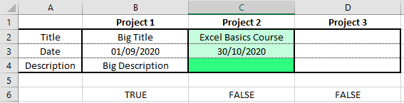
One thing I was needed to work out recently was how to make an Excel spreadsheet based form simple for others to fill in. This particular form spanned three pages, and included 191 items of information which needed to be filled in, plus various repeats and formulae and a chart of results. It was quite a hefty form, and I felt the need to provide some form of order to it.
What I ended up doing was selecting certain cells for different phases of the form. These made sense in my case for four different phases which may be completed at different times in the form’s lifecycle. Different people may fill each one out. What each phase had in common was that all of the information in that selection should be completed before the next phase was started.
So – colour coding is the obvious first step. The next leap in the design was to use conditional formatting to show which cells had and hadn’t been completed. The real kicker, though, was to have the different phases only light up when the previous ones were complete, but the current one was not. This really made a difference to the simplicity for my users. I’ll show you the steps needed to do the same thing for your spreadsheets, using a much simpler example.
Consider the following table – not hugely complex; just three items to be filled in. But imagine there were many, many items, and perhaps in different places on a spreadsheet, interspersed with formulae and lookups and images of technical stuff.
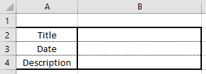
Colour-coding missing cells
Let’s add some colour coding to show the user which cells have been filled in, and which still need something adding.
- Highlight cells B2 to B4.
- Select Conditional Formatting -> New Rule from the Home menu.
- Click “Format only cells that contain”
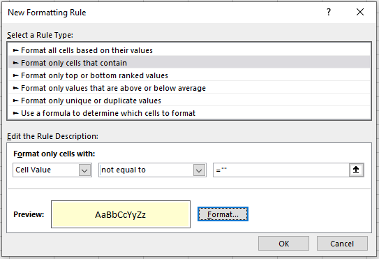
- Change the Rule Description to Cell Value -> equal to -> =””
- Click on Format and choose a format which will stand out and highlight the cell as being incomplete. Press OK.
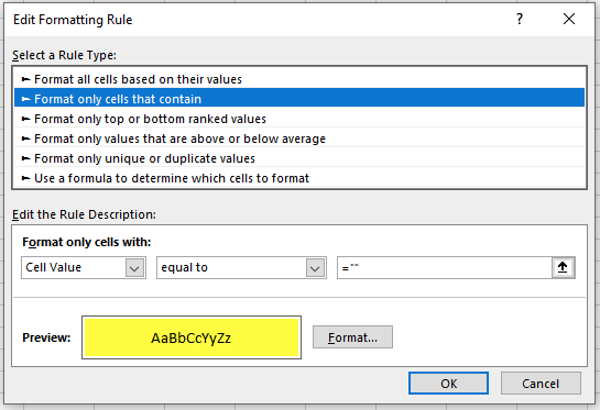
You should now see that all the cells you selected to have this conditional format are highlighted. Once you type something in, they will go back to white.
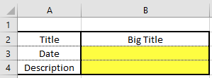
Colour-coding completed cells
That’s great, but if you want to show the cells which have had a user-entry already, you will want to highlight those in a different colour – perhaps a lighter shade of the first highlight. You could just colour these manually, and have them revert back to it when the highlight turns off, but that won’t work for the subsequent steps. So highlight them again, and click on Conditional Formatting -> New Rule again.
This will be just the same as the first one, except that we will set the Rule Description to read Cell Value -> not equal to -> =””, and the format will be different. Try a lighter shade.
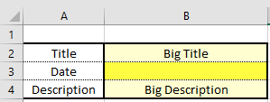
Now, when you put some data into those cells, they will remainin highlighted but change to a lighter shade.
Different colours for different sections
OK. Very good so far, but that’s not too complicated, is it? How about if I decide that the column B represents the first Project, and add a further two projects alongside it?

We might want to highlight each of those in a different pair of colours, to differentiate the different project phases. You can do this exactly the same way as the first Project, but highlighting each different set of cells and choosing different colours.
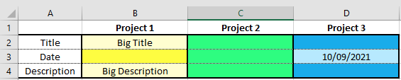
But now everything is highlighted all at once. The aim here was to have first Project 1, then Project 2, then Project 3 in turn. If it isn’t their turn, they should stay unshaded.
Colour coding dependant on current section
This is the clever part. We will need to find a way of determining when a Project is completed, and then build that into the conditional formatting. It is possible to do it all at once, certainly for this small example, but that isn’t very scaleable for complex spreadsheets, so we’ll do it in two parts.
First, we will add a formula in a different cell to work out if all of Project 1 has been completed. This could be on a different sheet, out of the way, but I’ll just put it beneath the Project column for now, in B16.
=IF(OR(ISBLANK(B2),ISBLANK(B3),ISBLANK(B4)),FALSE,TRUE)
For now it reads FALSE because not all of the cells are filled in. When you put something in all the cells, it will turn to TRUE.
Next we will revise the conditional formatting for Project 1. We need to tell the cells to only use that format if B6 is FALSE. If it is TRUE, we want the cells to remain unshaded, and we will tell Project 2 to light up instead.
Highlighted the cells you want to change and select Conditional Formatting -> Manage Rules. Select the first one and press Edit Rule.

For both of these rules we are going to change them in the same way. You need to change from the simpler rule type to the more versatile Use a formula to determine which cells to format option. Now we can put a variety of conditions in with a formula. Note the B2 – this is a relative cell reference and should be the same as the first cell in your highlighted range. $B$6 is the same cell that all of the range needs to refer to, so it is an absolute reference.
=AND(B2<>"",$B$6=FALSE)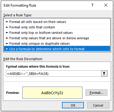
Press OK then do the same thing for the other format. This time the code will be:
=AND(B2="",$B$6=FALSE)Now, when all of the cells in that project have data in them, the highlighting will turn off. All that is needed now is to add summary boxes in cells C6 and D6, and modify the formats in a similar way.
In C6 and D6 put the following respectively:
=IF(OR(ISBLANK(C2),ISBLANK(C3),ISBLANK(C4)),FALSE,TRUE)
=IF(OR(ISBLANK(D2),ISBLANK(D3),ISBLANK(D4)),FALSE,TRUE)
Highlight Project 2 cells and change the conditional formatting to contain the following two formulae:
=AND(C2<>"",$B$6=TRUE,$C$6=FALSE)
=AND(C2="",$B$6=TRUE,$C$6=FALSE)
Highlight Project 3 cells and change the conditional formatting to contain the following two formulae:
=AND(D2<>"",$B$6=TRUE,$C$6=TRUE,$D$6=FALSE)
=AND(D2="",$B$6=TRUE,$C$6=TRUE,$D$6=FALSE)
You now have a completed form, which highlights the cells needing to be filled in, while showing the ones which have already been completed, for one phase after another in turn. As the form is completed the colour coding will progress to guide the user to where they need to go. Congratulations!