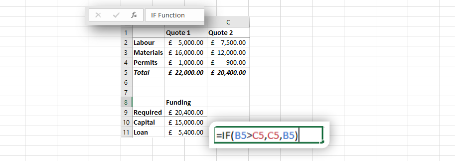
Excel is a very powerful tool – possibly one of the most powerful computer programs available to the casual PC user. Everybody who uses it knows that it can deal with lots of numbers and can give totals and averages, as well as charts to visualise the results. One very powerful function within Excel is the IF function, and its variations which give huge potential to Excel as a decision-making engine as well as just being a calculator.
How to use the Excel IF Function
Consider the following scenario. You are adding up two sets of data – possibly parts of two different quotes for work to be done. You would then choose the best quote and use that in further calculations – for example how much cash you need to find to fund the work.
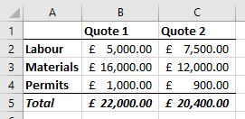
We have the two quotes in columns B and C. Each quote has the same items, but with different costs. The total in each column is a sum of the three cells above it. Nice and easy, and just like a calculator. The only benefit of using Excel so far is that it looks nice and the values can be altered to see the change in the total.
The next thing we need to do is to choose the better quote.
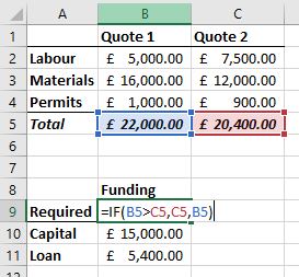
The function of choice here is the IF function. The syntax is fairly easy, and has three arguments:
=IF(expression, value if true, value if false)The first part is the expression which should be checked. This can be a comparison of different cells (B5 > C5 in this case) or it might be checking if a cell equals something. It could be a much more complex formula, and can be nested within other formulae as well.
The second part is the result if the expression is true. In this case we have said that B5 is greater than C5. If this is true then we want to have C5 in the cell (as this would be the cheaper quote). The third part is the result if false. In this case we want to show B5, which would then be the smaller value.
The beauty of this IF statement is that it chooses a value based on the criteria you have set. The spreadsheet can continue to make calculations based on that choice, and there is no need for additional human interaction. Obviously this is quite a simple use case, but the IF statement is a very powerful building block in the logic of Excel.
More Complex IF Functions in Excel
Consider this case:
=IF(ABS(costA - costB) <= 1000, IF(LeadtimeA <= LeadtimeB, SupplierA, SupplierB), IF(costA < costB, SupplierA, SupplierB)This piece of logic calculates the difference in two costs and checks if they are within £1000 of each other. If they are, then leadtime is the deciding factor instead. If they are not, then the cheaper cost wins. ABS, by the way, finds the absolute value. This is the value without a positive/negative sign, so it doesn’t matter which value was larger to begin with.
This formula also shows difference expressions which can be evaluated. <, >, =, <=, <> are all comparison operators which can be used. Expressions of multiple variables, functions, and ranges can all be used.
=IF(SUM(A1:A10)>=AVERAGE(B1:B10),"Larger Sum", "Larger Average")The results if true or false can also be functions, references, text, or a combination. They can be nested IF functions, as shown earlier as well.
Multiple criteria can be checked using the AND and OR functions.
=IF(AND(A1="Lemon", A1="Banana"),"Yellow fruit", "Not yellow fruit")The comparison operators do not need to be used if the expression results in a true or false without. For example, the value 0 is considered equal to FALSE in an IF function. Any other numeric value is TRUE, except #DIV/0. So =IF(0,”True”, “False”) returns False.
Other IF-Style Functions in Excel
There are other functions which incorporate the IF function.
IFS Function
This function allows multiple results apart from the two If TRUE and If False responses. Criteria are entered with the response if true following:
=IFS(A1="Apple","Fruit",A1="Steak","Meat",A1="Milk","Dairy",A1="","Enter a food")COUNTIF Function
The COUNTIF function will return the number of cells in a range which fulfil the criteria.
=COUNTIF(Range, Criteria)
=COUNTIF(A1:A10, "Apple")
The function above will count any cells in the range A1 to A10 which contain the word Apple.
SUMIF Function
This function is similar to COUNTIF, but instead of counting 1 each time a cell matches, it will add the corresponding value in a second range.
=SUMIF(A1:A10, "Apple", C1:C10)This function will look at A1 to A10 and every time the word Apple is found the corresponding value in C1 to C10 is added on.