
So, anybody who has dealt with Excel formulae between multiple sheets or tables is likely to know what VLOOKUP does. A few of these people have probably also used the similar HLOOKUP which searches along rows instead of down columns. Both of these functions have their place in Excel, and are relatively simple to use. In this article I’ll show you how to use VLOOKUP and what benefits using INDEX MATCH will give you.
How to use VLOOKUP
VLOOKUP is designed to search down the first column of a given range and then return the value in one of the other columns. This is great, and can work well.
VLOOKUP(lookup value, range, column number containing return value, type of match).The syntax above is fairly simple. The lookup value is the value (number, string or whatever) you want to find and match. The range is the range of values that you are matching and returning a value from. This should cover at least two columns therefore. In the example below the range highlighted is D4:F11.
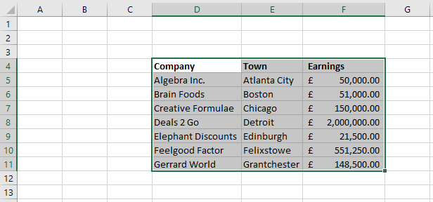
The column number is the number of the column within the range you’ve given. If the range started at A1, then this would relate to column A = 1, column B=2 and so on. But in the range above (and usually) column E is the second column and column F is the third column. In other words, it is relative to the column you are searching down, with the column you are searching being column 1.
The final part is optional, with a default of TRUE. If you leave it as it is, or put TRUE, the result will be an approximate match. This means that you have to have the values in order, and the search will return either the exact value or the one before where it would have been. This is the last value lower than the search item. If you put FALSE then it must return only the exact result, giving an error if the item isn’t in the search list.
=VLOOKUP("Gerrard World",D5:F11,2,FALSE)The formula above searches for Gerrard World in the first column of D5:F11, returning the result in the second column, and only returning anything if it can match the search string exactly. It returns Grantchester.
=VLOOKUP("Algebra Ltd",D5:F11,3,FALSE)Whereas the formula above searches for Algebra Ltd or the nearest result (before) to it. It returns the value in the third column of the range. Algebra Ltd isn’t in the list, but it finds Algebra Inc. instead. It returns 50000.
All well and good – HLOOKUP works in the same way except it searches rows instead of columns. If you are working with these functions already, and not noticing any issues, then you are likely to be able to continue without looking at improvements. However, there are a few issues with these lookup functions:
Problems with VLOOKUP
Fixed Column References
You may have noticed that when you use Excel’s excellent formula-drag feature the column numbers in the third argument do not change. This can be a real disadvantage when creating large tables of values where normally the absolute/relative cell referencing can be worked in your favour. It also doesn’t update if the data itself moves. Usually with most formulae they will follow the cells that they refer to and change to suit when they move.
Inserting Columns Destroys your Formula
In a similar manner to the previous point, if you insert a column into the datarange, the range itself will update but the column being returned will not. Therefore you will start getting data which is not what you asked for. If you add a column at the end of the table the range won’t update either.
Only Lookups from Left to Right
The biggest issue with the lookup functions is that they can only search down the first (left-hand) column of your range, and then return a value to the right of that. This is no good if you want to vary which data you search for, and you will end up adding extra columns which copy the data.
Try finding the company name which operates from Detroit in the example table. You will find that you want to have columns D, E and possibly F in the range, but it will only search in the left-hand column, D. You will need to set the range to column E through G and put a formula in column G which copies column D, the company name (or a similar arrangement).
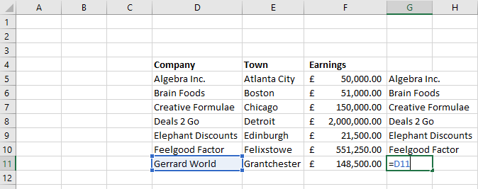

This is a convoluted way of cross-referencing the data, and can end up in doubling the number of columns required.
Processing Power
The lookup functions use a significant amount of processing power. This is less noticeable in modern versions of Excel, but there is still potentially a lot of data, all of which needs to be examined, in every column, by Excel.
Improvements with INDEX MATCH
The solution to all of these problems is INDEX MATCH. This is a duo of functions which complement each other perfectly, and are commonly used together to create a more functional VLOOKUP function. It is a slightly more complex looking function, but is relatively simple to remember if you use it a lot. The generic structure is this:
=INDEX(Return value range, MATCH(Lookup value, Search range, match type))This structure looks longer, but there are actually exactly the same number of variable, and they are the same ones, practically. The difference in the variables is that it is two columns (or rows, or a combination) which are selected separately rather than one big range from which a specific column number is chosen. The match type is slightly different to the VLOOKUP one, being either 1 (the largest value less than or equal to the lookup value), 0 (the exact lookup value), or -1 (the smallest value greater or equal to the lookup value). I always use 0.
To use this with the very first example on this article, finding the city that Gerrard World operates in, use the syntax below:
=INDEX(E5:E11,MATCH(D15,D5:D11,0))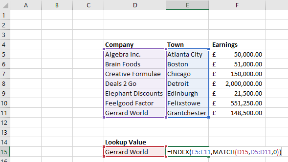
To understand how this works, we can split it into the two separate functions.
INDEX returns the value at a given position in a range. For a single column, or a single row, just one value is needed and it gives the value at that position in the column or row. So doing INDEX(D5:D11,5) on the table above gives us the 5th value in the range D5:D11 – Edinburgh. For the INDEX MATCH method, the position of the value is given by the MATCH function.
MATCH returns the position of a value in a range which matches the lookup value. So using MATCH(“Chicago”,E5:E11,0) gives the position of the word CHICAGO in that range, which is 3 (the 3rd cell in the range).
Putting these together means that we can search one range to find the position of the value using MATCH, and pass that position to the INDEX function to return the value in the same position in a different column.
Benefits of INDEX MATCH
The benefits of using INDEX MATCH are apparent when you examine the formulae.
- Firstly there are no numeric values which reference the ranges, as in the column number of the VLOOKUP function. You will find that if you move ranges around, or drag and copy formulae, the ranges keep track and remain correct.
- Secondly there is no dependence on a single range, so additional columns are not a problem. Each column you are referencing is identified in the formula, and will remain correct no matter what happens. In fact, even if the ranges become completely decoupled, or occupy different worksheets, the formula will still work correctly.
- Thirdly, as a corollary of the second point, you will find that it does not matter which way you are reading the data across. You can lookup from left to right, or right to left, or even from a column to a row or vice versa if you like! This is probably the largest benefit of this function.
- Finally, there is some performance benefit, as the function only uses the data from the two columns, and not a whole range of data between them.
Conclusion
In summary, there are a number of key benefits of using INDEX MATCH over VLOOKUP, and the only downside is that the formula looks slightly more complex. It is dramatically more powerful, especially when used in more complex spreadsheets where the values are programatically created. It is also far less likely to lose its data when the ranges change.
There are improvements which Microsoft have made to their lookup functions. XLOOKUP and XMATCH are improved functions which remove some of the limitations described. However these still pale in comparison to INDEX MATCH in most scenarios.